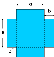
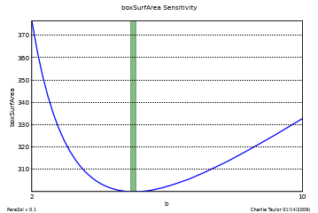
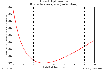
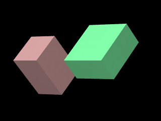
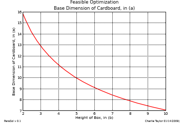
Example 3 optimizes a cardboard box.

This is "almost" problem 12 in Chapter 10 of the book "Numerical Methods in Engineering with Python" by Jaan Kiusalaas. The task is to minimize the amount of cardboard required to build an open topped box with a volume of 500 cubic inches.

Volume = 500 in³
find a and b with minimum surface area.

parasol is capable of operating on much larger models, however, this demonstrates a model with several inputs, outputs, and constraints.

Two solutions will be demonstrated and both will find the answer to be a = 10 inches, b = 5 inches.

The first solution simply gives "a" and "b" as inputs, "Volume" and "boxSurfArea" as outputs, applies the 500 in³ constraint to Volume, and minimizes boxSurfArea by changing both "a" and "b".(click herefor first solution source)

The second approach uses a parsol feature called "Feasible Pairs". A feasible pair is one input variable, one output variable and a desired value for the output variable. At each call of the control routine, the value of the input variable is found that results in the desired output value.

In this case for example, at each evaluation, the value of "a" is found that results in "Volume" being 500 in³. This effectively changes the problem from being two dimensional in "a" and "b", to being one dimensional in "b" only.

It is called a feasible pair because only feasible values of Volume are considered. (for second solution sourceclick here)

The feasible pair algorithm is implemented by using a root solver to iterate the value of "a" and solve for the desired value of "Volume" using the current value of "b". It uses the very efficient algorithm by Jack W. Crenshaw "A root finder's roots".

The second solution approach will also demonstrate the Persistance of Vision ray tracing software and how it can be used to illustrate a 3D physical result.

Both of these parasol files begin very much like Example 2 (i.e. There are two input variables and two output variables). Since the first approach is so much like Example 2, I will focus on the feasible pair approach.

Notice that there are two new imports in the file to support POV ray tracing.

from parasol import *
from parasol import POV_Basics
from parasol import POV_Items

PrDesc = ProblemDescription(taskName="Best Box",
    subtaskName="Feasible Optimization", author="Charlie Taylor")

# design vars have: 
#     name, value, minVal, maxVal, NSteps,  units,  description
PrDesc.addDesVars(
    ['a',12,1,50,50,'in','Base Dimension of Cardboard'],
    ['b',10,2,10,50,'in','Height of Box'],
    )

# result variables have: 
#    name,      units,  description 
PrDesc.addResultVars(
    ['Volume','cuin','Box Volume'],
    ['boxSurfArea','sqin','Box Surface Area'],
    )

There is nothing suprising in the control routine. It is like the other examples we have seen.

# the following control routine ties together the system result variables
#  with the system design variables
def myControlRoutine(PS):
    # get current values of design variables    
    a,b = PS("a","b")

    # calculate result variables
    Volume = b * a**2
    boxSurfArea = 4.0*b*a + a**2

    # set output variable values
    PS["boxSurfArea"] = boxSurfArea
    PS["Volume"] = Volume

When using POV to render a 3D image, we must create a render control routine and give the ProblemDescription object the name of that render control routine (myRenderControlRoutine). In this case, the render control routine takes the initial values of a and b (global variables aInit and bInit) and shows that initial box in pink. Next to the original pink box, it renders the current values of a and b as an aquamarine box. We will call the render routine after optimization in order to show the best box next to the original box.

def myRenderControlRoutine(PS):
    a,b = PS("a","b")

    b1 = POV_Items.Box(corner1=[0,0,0], corner2=[aInit,aInit,bInit],
        texture=POV_Basics.Texture( colorName="Pink", ambient=0.5 ) )

    offset = max(aInit, bInit) * 1.5

    b2 = POV_Items.Box(corner1=[offset,0,0], corner2=[offset+a,a,b],
        texture=POV_Basics.Texture( colorName="Aquamarine", ambient=0.5 ) )
    return [b1, b2]

# need to tell system the name of the control routine
PrDesc.setControlRoutine(myControlRoutine)
PrDesc.setRenderControlRoutine(myRenderControlRoutine)

PS = ParametricSoln(probDesc=PrDesc)

Here is where we define our feasible pair. This "makeFeasiblePair" command simply says that our output variable is "Volume", its feasible value is 500.0, and that the input variable "a" is used to control the value of Volume. The defined range of "a" will be used as the search range to solve for Volume = 500 in³. (The range was defined as 1 to 50 in the above "addDesVars" command)

PS.makeFeasiblePair( outName="Volume", feasibleVal=500.0, inpName='a')

The code below makes one call to the control routine, saves the initial values of a and b, and saves a summary of the initial design. These values of aInit and bInit will later be used in the render control routine.

PS.evaluate()
aInit,bInit = PS("a","b")
PS.saveFullSummary()

The remaining code minimizes the box surface area by finding the best value of "b", creates a 3D image of before and after, makes some plots to help visualize the results, and saves a summary of the optimized box. This example also introduces a sensitivity plot to display results

# now optimize the system.
minimize(PS, figureOfMerit="boxSurfArea", desVars=[ 'b'], MaxLoop=500)

PS.render(view='front',ortho=1)

makeSensitivityPlot(PS, figureOfMerit="boxSurfArea", desVars=['b'])
make2DPlot(PS, sysParam=['boxSurfArea'], desVar='b')
make2DPlot(PS, sysParam=['a'], desVar='b')

# now save summary of system
PS.saveFullSummary()

Like all other examples, the last task is to tell parasol to finalize the output and close all files.

PS.close()  # finish up with output files

The output from the minimize operation is shown below. It shows that at the starting value for b of 10, and the boxSurfArea value was 332.843. The optimizer improved that to a value of 300 by changing b to 5. The parasol HTML output file contains the table shown below.

ParametricSoln: Feasible Optimization
            
====================== OPTIMIZATION DESIGN VARIABLES =======================
      name         value        minimum   maximum
         b           10            2           10 Height of Box  (in)

 Figure of Merit: Box Surface Area (boxSurfArea) = 332.843 sqin <== Minimize
============================================================================

ParametricSoln: Feasible Optimization
            
====================== OPTIMIZATION DESIGN VARIABLES =======================
      name         value        minimum   maximum
         b            5            2           10 Height of Box  (in)

 Figure of Merit: Box Surface Area (boxSurfArea) = 300 sqin <== Minimize
============================================================================

To verify the above results, curves of boxSurfArea vs b are shown below (click them to enlarge). The plot on the upper left is a sensitivity plot showing the current design point with a vertical green line. (Typically, more than one design variable is shown on a sensitivity plot) The plot on the upper right is a standard 2D plot of boxSurfArea vs b (no design point shown). The plot on the lower right is the value of "a" required to give 500 in3 vs "b". The POV rendering in the lower left shows the original box in pink and the optimal box in aquamarine.

To view HTML output from Example 3 Simple Method click here

To view HTML output from Example 3 Feasible Pair click here

Colorized listings thanks to ASPN Recipe at http://aspn.activestate.com/ASPN/Cookbook/Python/Recipe/442482 by Peter Krantz