Example 2 is a constrained function minimization.

This is problem 6 in Chapter 10 of the book "Numerical Methods in Engineering with Python" by Jaan Kiusalaas. The task is to minimize the function F(x,y) where x+y <= 1 and x >= 0.6

F(x,y) = (x-1)² + (y-1)²
    where:    x+y <= 1
    and:      x >= 0.6

While this example only operates on a simple function, parasol is capable of operating on very large math models with many inputs, outputs, and constraints.

The parasol file begins very much as in Example 1, except that there is a second result variable "sumXY" and a limit placed on the result variable "sumXY". The setResultVariableLimits statement sets a high limit of 1.0 to satisfy the x+y <= 1 constraint. (to download the source click here)

The addDesVars statement sets the minimum value of x to 0.6 to satisfy the constraint x >= 0.6. Since x+y <= 1 that implies a maximum value for y of 0.4.

from parasol import *

PrDesc = ProblemDescription(taskName="Minimize F(x,y) with x>=0.6 and x+y<=1",
    subtaskName="F(x,y)=(x-1)^2 + (y-1)^2",
    author="Charlie Taylor")

# design vars have: 
#     name, value, minVal, maxVal, NSteps,  units,  description
PrDesc.addDesVars(
    ['x',0.6,.6,1.,50,'','X value'],
    ['y',0.2,-0.2,0.4,50,'','Y value'],
    )

# result variables have: 
#    name,      units,  description 
PrDesc.addResultVars(
    ['F','','Function Value'],
    ['sumXY','','Sum of X and Y'],
    )

PrDesc.setResultVariableLimits(name="sumXY", hiLimit=1.)

The control routine is much like Example 1 except there is a second result variable to assign (A more complex problem would typically import a large math model).

# the following control routine ties together the system result variables
#  with the system design variables
def myControlRoutine(PS):
    # get current values of design variables    
    x,y = PS("x","y")
    # set output variable values
    PS["F"] = (x-1.)**2 + (y-1.)**2
    PS["sumXY"] = x + y

As in Example 1, the final tasks required for the setup are to give the ProblemDescription object the name of the control routine (myControlRoutine) and to create the parasol object (PS).

# need to tell system the name of the control routine
PrDesc.setControlRoutine(myControlRoutine)

PS = ParametricSoln(probDesc=PrDesc)

Again like Example 1, the statements below minimize "F", save a summary, and make some plots to help visualize the results. This example introduces a carpet plot to display results

# now optimize the system.
minimize(PS, figureOfMerit="F", desVars=[ 'x','y'], MaxLoop=500)

# now save summary of system
PS.saveFullSummary()

makeCarpetPlot(PS, sysParam="F", xResultVar="sumXY",
    desVarL=[["x",0.6,0.8,1.0],["y",0.0,0.2,0.4]], angDesVarL=[40,0])

makeContourPlot(PS, sysParam="sumXY", desVars=["x","y"])

makeContourPlot(PS, sysParam="F", desVars=["x","y"])

Again like Example 1, the only remaining task is to tell parasol to finalize the output and close all files.

PS.close()  # finish up with output files

The output from the minimize operation is shown below. It shows that at the starting values for x and y of 0.6 and 0.2, the function value was 0.8. It also shows that the constraint that x+y <= 1 is more that satisfied by a value of 0.8.

The optimizer improved that to a value of 0.52 by changing x and y to 0.6 and 0.4 respectively. This had the effect of running the value of x+y right up to the constraint value of 1. The table below can be seen in the parasol output by opening the HTML output file that parasol creates.

ParametricSoln: F(x,y)=(x-1)^2 + (y-1)^2
            
====================== OPTIMIZATION DESIGN VARIABLES =======================
      name         value        minimum   maximum
         x          0.6          0.6            1 X value
         y          0.2         -0.2          0.4 Y value

 Figure of Merit: Function Value (F) = 0.8  <== Minimize

========================== OPTIMIZATION CONSTRAINTS =========================
      name         value        minimum   maximum
     sumXY          0.8 ------------            1 Sum of X and Y
============================================================================

ParametricSoln: F(x,y)=(x-1)^2 + (y-1)^2
            
====================== OPTIMIZATION DESIGN VARIABLES =======================
      name         value        minimum   maximum
         x          0.6          0.6            1 X value
         y          0.4         -0.2          0.4 Y value

 Figure of Merit: Function Value (F) = 0.52  <== Minimize

========================== OPTIMIZATION CONSTRAINTS =========================
      name         value        minimum   maximum
     sumXY            1 ------------            1 Sum of X and Y
============================================================================

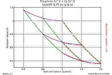
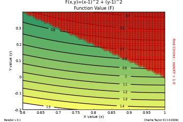
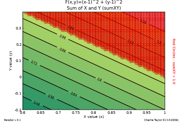
To verify the above results, 2 contour plots and a carpet plot were made (click them to enlarge). Those plots are shown below. The red dots on the various plots are locations where the constraint was violated (i.e. x+y > 1). The carpet plot is probably the most illustrative of the constraint impact on the function minimum. The sum of x+y is shown on the X axis and the function value is shown on the Y axis. There are contours of constant values for x and y (x in green, y in purple).

To view HTML output from Example 2 click here

Colorized listings thanks to ASPN Recipe at http://aspn.activestate.com/ASPN/Cookbook/Python/Recipe/442482 by Peter Krantz